CQF talk on a quantum view of Black-Scholes

It was a pleasure speaking yesterday at the Quant Insights conference marking the 50th anniversary of the Black-Scholes model. My talk presented nine predictions which came out of the quantum model – things that I had not been aware of, but that were suggested by the model and proved correct after empirical tests. And they all had implications for option pricing and the Black-Scholes model.

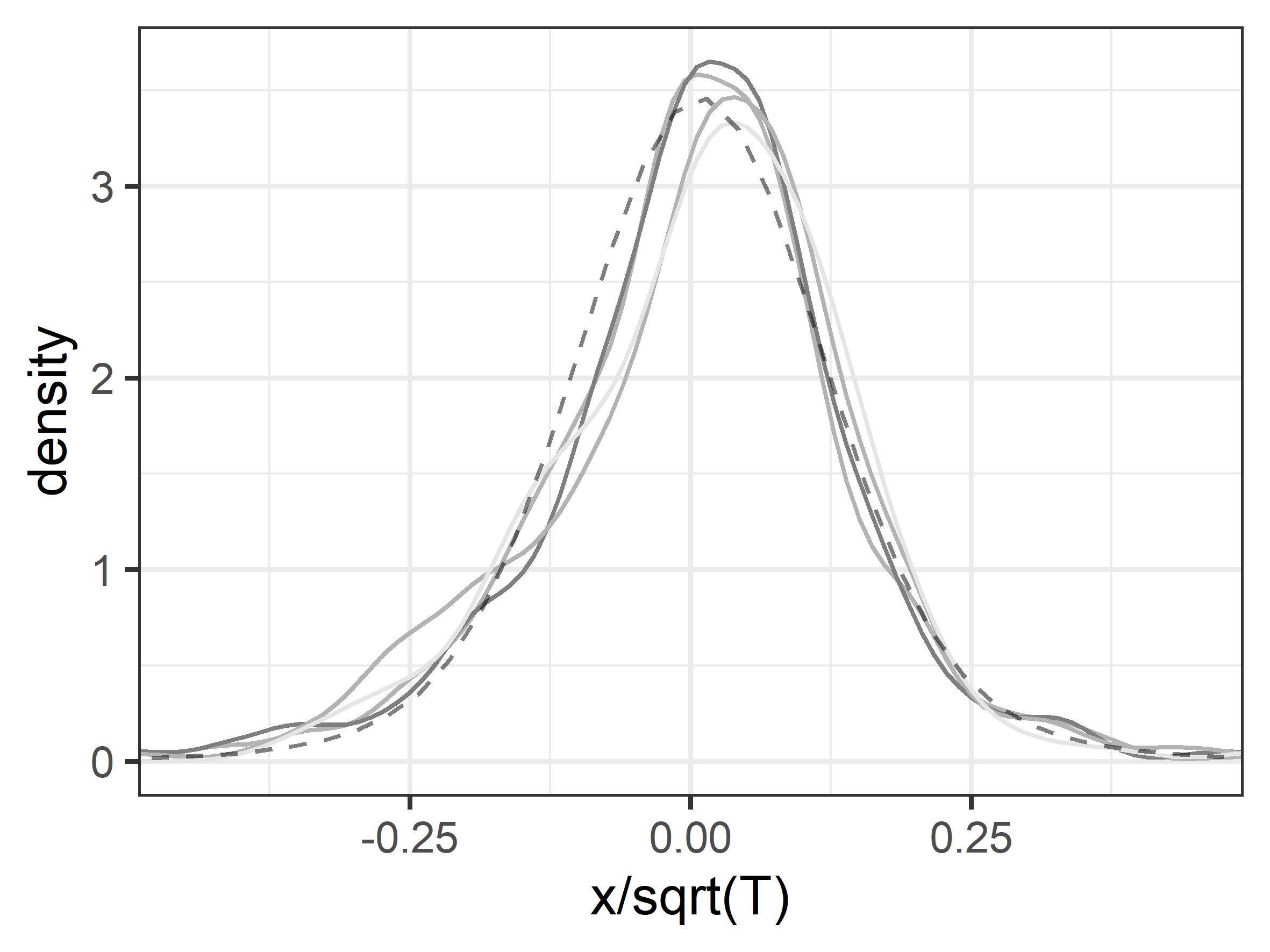
1. Before starting to work with the model, I didn’t know that price change and volatility for index data such as the S&P 500 or DJIA scale inversely with the square-root of time, even though the price change data is not normal, and volatility is not constant.

Density plots of log price changes, normalized by the square-root of time in years, for the S&P 500 over the years 1992-2021. The solid lines, from darkest to lightest shades of grey, are for periods of 1, 2, 4 and 8 weeks (measured in days). Dashed line is the quantum model.

2. I had heard of the square-root law of price impact, which says that the price change induced by a large order scales with the square-root of the order size, but didn’t know that the numerical coefficient was approximately one, as predicted by the quantum model.

Plot of price change versus order size Q over average daily volume V follows a square-root law with coefficient near unity.

3. I certainly didn’t know that the variance followed a simple equation that contradicted a published result.

Variance plotted against imbalance Q/(VT) where Q is order size, V is daily volume, and order time T ranges from 3.5 minutes (black) to 345 minutes (light grey). The single parameter sigma estimates the volatility.

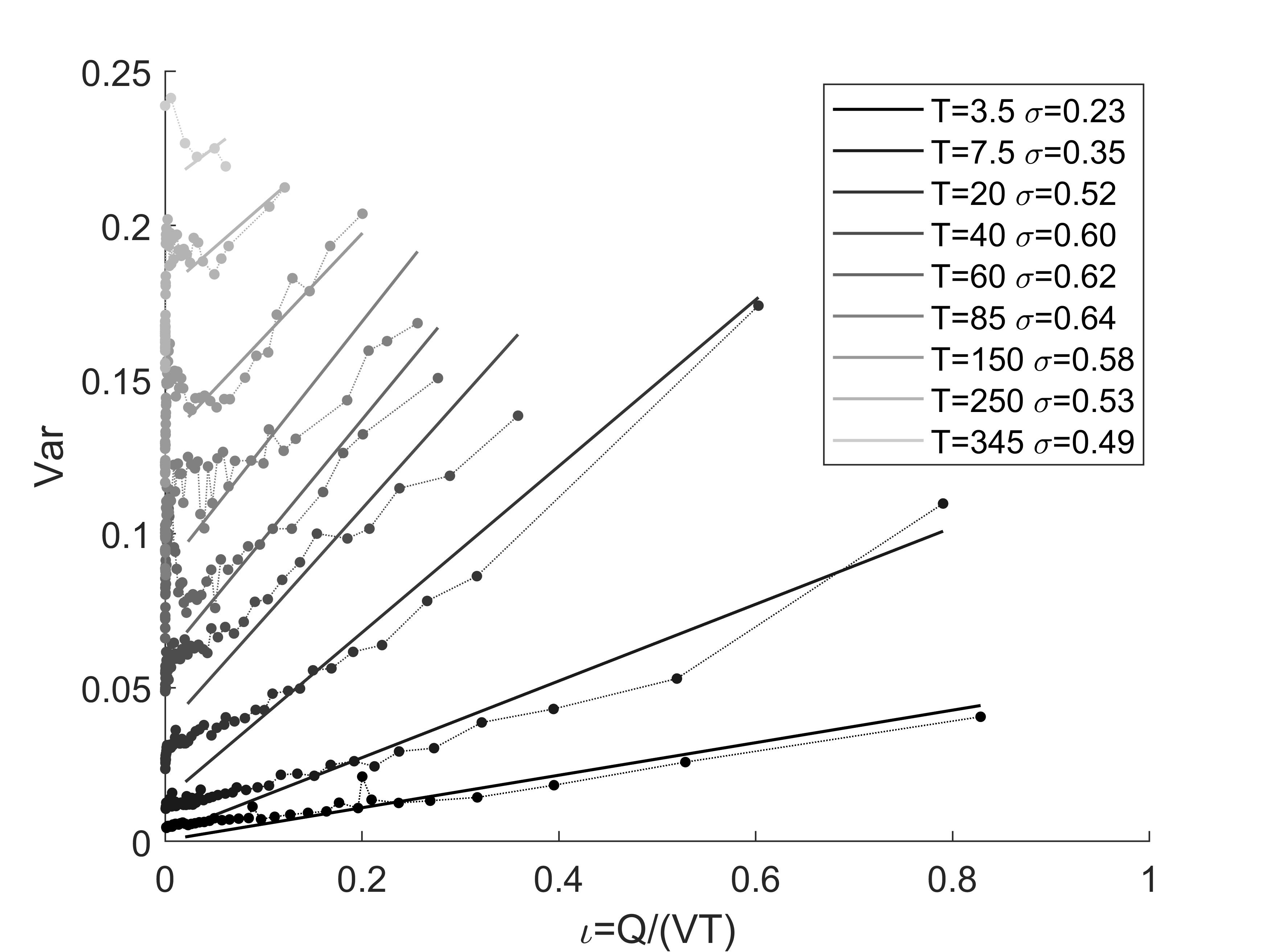
The drawbacks of the neoclassical model of supply and demand have long been pointed out by critics such as Steve Keen. A basic one is that what counts is not supply and demand separately, but the ratio of demand to supply for available units. The quantum price impact model therefore gives an alternative model with only a single parameter, that has been rigorously tested for stock market data.

Plot of log price against imbalance, which is the ratio of demand to supply per available unit.

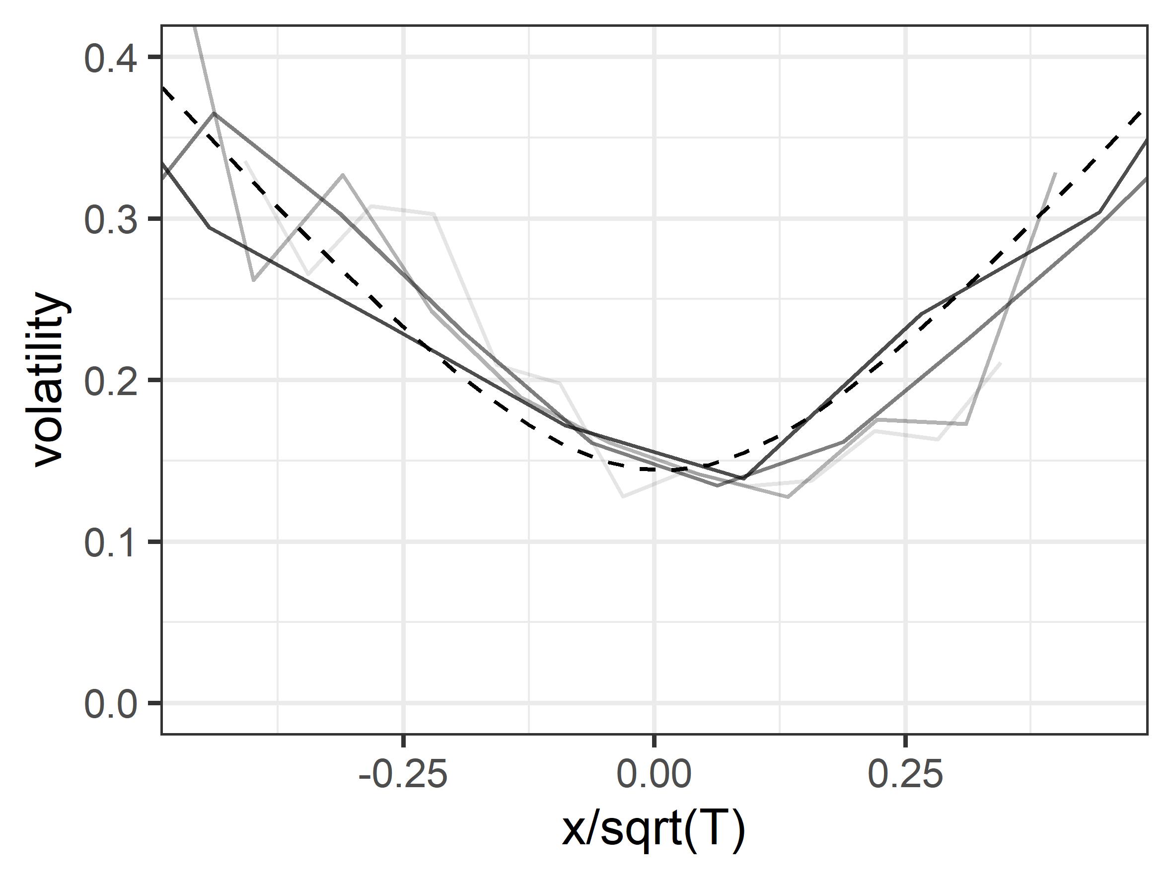
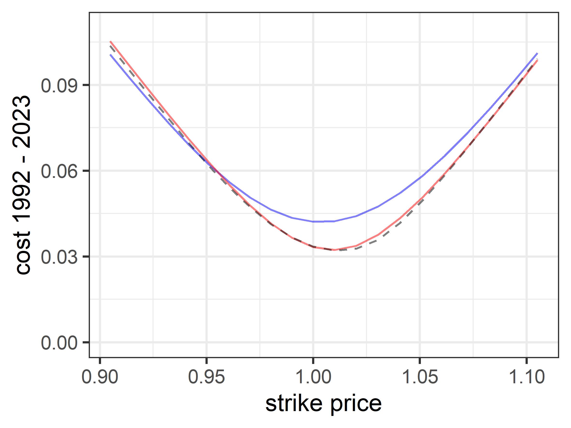
4. I had heard of the implied volatility smile in options trading, but didn’t know that actual volatility showed an even more pronounced smile, that followed a simple relationship with price change and time (and is related to price impact). I’m sure I am not the first person to notice this fact, but I haven’t seen it, or the connection with implied volatility, reported in the literature.

RMS annualized volatility for the S&P 500, plotted against normalized price change, for periods of 1, 2, 4 and 8 weeks (dark to light). Dashed line is the quantum prediction.

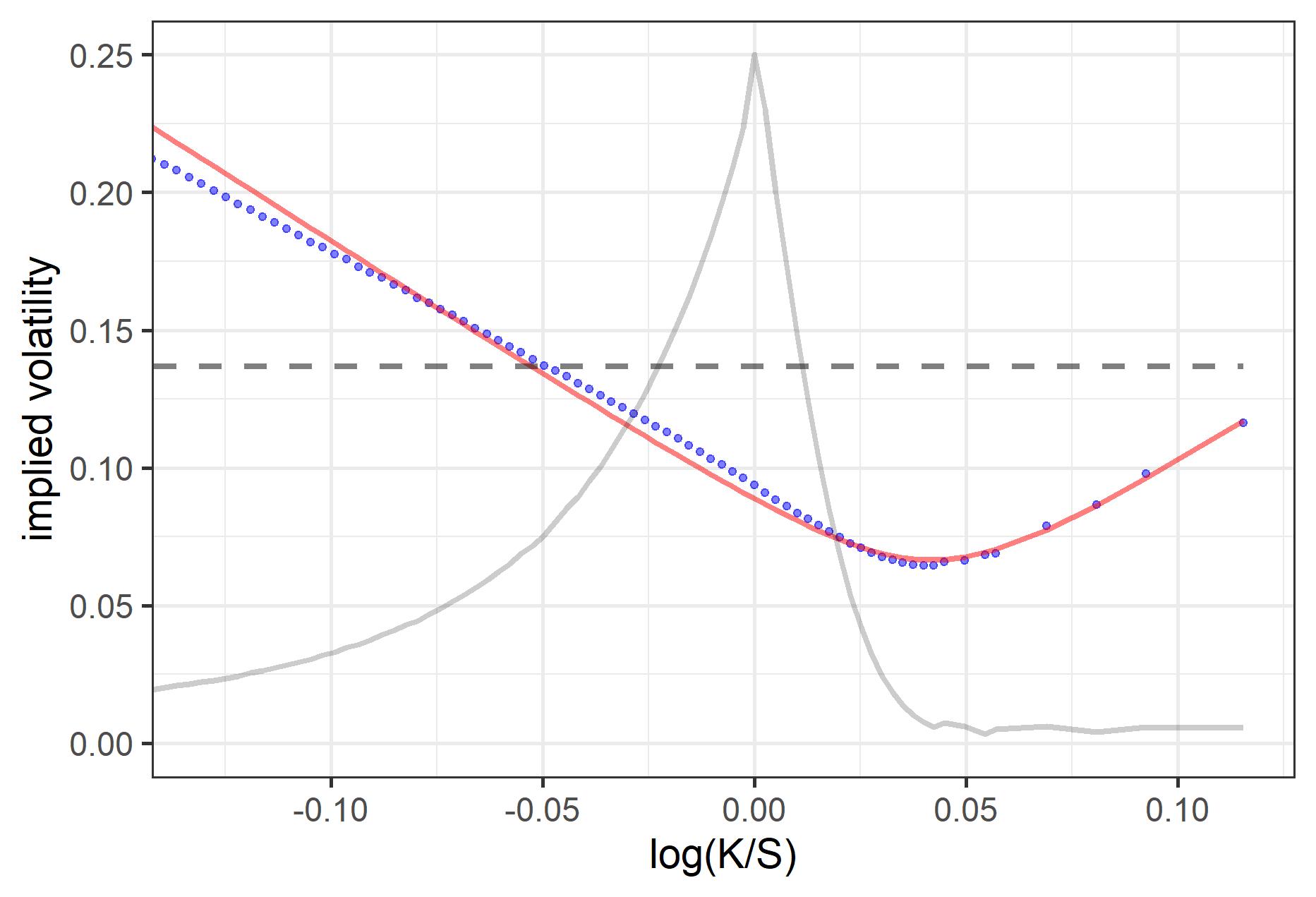
5. Implied volatility is not the same as actual volatility, because it is found by fitting a lognormal option pricing model to data that is not actually lognormal, and is affected by trader behaviour. So it was interesting to find that the quantum model produced an implied volatility surface very similar to what is found in the wild.

The quantum implied volatility surface is a somewhat flattened version of actual volatility.

6. The VIX index is an estimate of future volatility based on implied volatility, which is in turn used to price other options. The VIX is often described as being model independent, but its formula is based on two things: that volatility is independent of strike, and that the relevant growth rate is the risk-free rate. The former is an assumption of the Black-Scholes model, while the latter is its key finding. The VIX is therefore Black-Scholes in another guise. The quantum model predicted that the VIX substantially over-estimates both implied volatility and actual volatility, because its formula adds up the contributions of options in the wrong way. The results agree.

The VIX is produced using a formula which assigns weights to options (grey line) and produces a single volatility (dashed line) which is supposed to represent the implied volatilities (blue points). The quantum model (red) is a version of the smile curve.

7. Given that the Black-Scholes model assumes constant volatility, it makes sense that it should misprice options. However I for one was surprised to find that, according to the quantum model, it misprices at-the-money straddle options by a factor about equal to the square-root of two.

Comparison of straddle option pay-in for Black-Scholes model (blue) and quantum model (red), with expected pay-out (dashed). The Black-Scholes model misprices at-the-money straddles by about 40 percent.

8. Since the Black-Scholes model is the industry-standard pricing model, it makes sense that model error will lead to mispricing in option markets. This prediction was verified by Larry Richards who analyzed CBOE data for over 25,000 1-month SPX option prices from 2004 to 2017. So much for efficient markets. See our paper published in the March 2023 issue of Wilmott.

9. Finally, a logical consequence of this is that one can devise options-trading strategies to exploit this mispricing – for example, by selling at-the-money straddles (with appropriate protection to cover potential losses).

To summarise, the main difference between the classical random walk model traditionally used in quantitative finance, and the quantum model, is that the former assumes markets are at equilibrium and volatility is constant, while the latter treats markets as a dynamical system where price change and volatility are linked. The quantum model therefore does a better match of fitting and predicting market behaviour, without relying on additional made-up parameters of the sort so common in traditional quant finance.

In a panel discussion in which quants Emanuel Derman and Robert Litterman reminisced about the history of the Black-Scholes model, a viewer asked Derman whether “quantum economics and finance was too much of a stretch.” He agreed (again, predictably) that yes it was, without giving specific reasons (though he added that he would be willing to reconsider). And yet it’s strange that previous studies of implied volatility – including Derman’s own book The Volatility Smile – didn’t pick up on the obvious fact that the implied volatility smile is a weaker version of a smile seen in the actual asset price data (see my article The Black-Scholes Magic Trick in the July 2023 issue of Wilmott). Or that this would lead to a significant mispricing of commonly-traded options.

Models aren’t just tools to analyze systems, they also affect what we do and don’t see. And in finance, the quantum model isn’t too much of a stretch – it’s a perfect fit. For details of the quantum model, see here. And for more work along these lines, please follow our new journal Quantum Economics and Finance.

Update: A video of the talk is now available for members (free) at the CQF Institute website (see Part 3). See also the related paper “Quantum Uncertainty and the Black-Scholes Formula” available at SSRN.