The quantum implied volatility model

The quantum implied volatility (QIV) model is a minimalistic model of an implied volatility surface. The aim is to capture the main features of implied volatility using a small number of parameters.

The model is derived by assuming that the implied volatility is the volatility which, when used as input to the Black-Scholes model, will produce the correct option price under the quantum model of asset price. Let x be log price change over a period T, and set z=x/√T. If we ignore the drift term, the quantum model then says that the price distribution can be modelled as a Poisson-weighted sum of Gaussians in z. If we now calculate the volatility which gives the correct option price for that distribution, then we find it satisfies

where again z=x/√T but now x represents log moneyness (see here for derivation). The only parameters are a base volatility s, and the number q which has a typical value of about 0.95.

The QIV model was tested against SPX options during the period 2004-2020. The results are shown in the figures below. The left panel shows implied volatility as a function of T and z=x/√T (chosen because the quantum model is expressed in terms of z). The option prices are averaged over each strike and expiration (from five days to one year), and the implied volatility is then computed. Put options are used for x<0 and calls for x≥0. The quantum model is shown by the red line. The right panel is an end view of the same data, which shows that the surface is independent of the period T when plotted in this way.

The results are not perfect, especially for at-the-money options, which is not surprising given that implied volatility is complicated by a number of behavioural and other effects. For example, for z near zero, put options (to the left) attract a higher price than call options (to the right). However the quantum model correctly predicts the overall V-shaped configuration that appears when the data is plotted in this way, and does a better job at more extreme strikes. Results could obviously be improved by adding more parameters, but the aim here is to show that the surface can be fit quite well using only the basic model with q=0.95.

Also, it should be noted that the QIV model is a prescriptive model, in the sense that it calculates the correct volatility to use given a quantum price distribution. If traders are using a significantly different implied volatility, then that may suggest a degree of mispricing, and therefore an opportunity for arbitrage.

For details and other applications of the model, see the paper “A quantum model of implied volatility” in the May 2024 issue of Wilmott. A pre-publication draft is also available here.

Quantum economics – real or fake?

Since I started working in quantum economics, a persistent problem was finding suitable venues for publication. Journals in economics or finance wanted nothing to do with it (the exception was Wilmott magazine), so most papers were published in physics journals like Physica A, which meant that no one working in economics ever heard about them. The field clearly needed its own journal! A few years later, with help from many people and Sage Publications, Quantum Economics and Finance was launched.

While my motivation for co-founding the journal was because I wanted the field to succeed, I’ll also admit that there was a selfish interest in that I thought it would give me somewhere to publish my own work – which for some reason often fails to find a home. However it turns out that my papers are so weird, that they are rejected even by my own journal.

The first paper to run into trouble was “A Quantum Oscillator Model of Stock Markets”. One of the main findings is that volatility over a period T is described by the equation

where x is log price change over the same period, adjusted for average drift. The equation was a prediction from the quantum model, and it turned out to hold surprisingly well for a range of asset types including stock market index price data (see figure below for the S&P 500). The formula is useful because it leads to a minimalistic two-parameter model for the implied volatility surface.

RMS annualized volatility plotted against normalized price change for the S&P 500. The solid lines, from darkest to lightest shades of grey, are for periods of 1, 2, 4 and 8 weeks. Dashed line is the quantum model. Figure from A Quantum Oscillator Model of Stock Markets.

What makes the above equation a falsifiable prediction rather than a curve-fitting exercise is that (a) I had no idea it was valid until I tested it and (b) it does not involve any extra parameters, other than a base volatility. Yet when I submitted the paper for review – again, in my own journal! – neither reviewer showed interest in the equation, or its success in modelling empirical price data.

One reviewer in particular wasn’t having it. As they wrote: “the modeling methodology is not appealing. A mass parameter, a fake Plank [sic] constant, and a frequency are introduced to finally describe a quadratic behavior … It is hard to believe that a classical model cannot reproduce the same. Am I right?”

The reviewer here was talking about parameters from different parts of the paper which had no effect on the equation, whose sole parameter is the base volatility. Perhaps they would have found an equation with zero parameters more appealing, less fake?

The paper went to a tie-breaker, who backed publication. Phew!

Next up, “Blinded by Science: The Empirical Case for Quantum Models in Finance”. The theme of this follow-up paper was that people working in economics and finance systematically ignore – or simply do not see – empirical evidence that doesn’t fit their classical assumptions, such as the no-arbitrage principle.

Reviewer 1 nailed the “do not see” thesis right off the bat by stating: “I do not see the point of the paper.” It turned out there was a lot more they didn’t see.

The paper brought out the same equation and pointed out that it was a new finding. The reviewer shot that down by saying that “many models … have considered non-constant volatility.” They were therefore “very confused” by the claim that this was a new result.

On then to Reviewer 2 who wrote that: “This stylized fact is well known … So there is nothing new here … No, nothing leads to this equation which is a purely arbitrary choice of the author, and nothing guarantees that in practice volatility follows [it] (and it is of course not the case).”

So to summarise, the equation is not a prediction, it’s a stylized fact and a purely arbitrary choice which is nothing new and of course not the case and everyone knows it except they don’t because it’s wrong anyway.

The reviewer then swivels their laser-like focus to the somewhat peripheral topic of music theory, because I had remarked as an aside that the energy eigenvalues of the oscillator have frequency ratios of 1, 3, 5 so the tone produced is a major chord. The reviewer set me straight: “it is true that a major chord is composed a the tonic (1), major third (3) and dominant (5), but this has nothing to do with frequencies, only with the position of the notes in the diatonic scale – and actually there are 2 tones between 1 and 3 and 1.5 tone between 3 and 5, therefore the frequency ratios are absolutely not 1, 3 and 5.”

It seemed telling that even for this, a reviewer would rather trust their hazy understanding of theory rather than look at something real, like an actual guitar. A major C chord has notes C, G and E. So if you play these notes, it gives a major C chord:
  Note Frequency Ratio to C1
  C1  32.703   
  G2  97.999   2.996636
  E3  164.81   5.039599

The other critiques of the paper were no more coherent. One bizarrely insisted that I had mistaken volatility for its square, the variance, perhaps because they “could not see” a square-root sign in front of it.

Apparently there is a new form of therapy called “rejection therapy” where people are counselled to deliberately seek out situations where they are rejected, as a way to build robustness and lose their fear of failure. Quantum economics has certainly proved fruitful as a way to have my work rejected in new and surprising ways, with untold therapeutic benefits.

On a more serious note, though, I think this shows the difficulty in getting new ideas accepted in science, especially if they are in conflict with mainstream results. I have prior form in this area, since I did my D.Phil. on model error in weather forecasting and found it almost impossible to publish papers which pointed out the limitations of weather models. As I wrote in my 2007 book Apollo’s Arrow, a typical pattern was illustrated by one research head who “claimed the research both showed nothing new, and ‘flies in the face of most of the available experimental evidence’.”

I have no idea who the anonymous reviewers for Quantum Economics and Finance were, and because the paper was rejected I didn’t get the chance to respond to them (until now!). But the thing I found strangest about these reviews was that at no point did the reviewers engage with the empirical evidence. It was another example of how experts “do not see” data which contradict longstanding assumptions based on classical theory. They just stated (as one put it) that “there is nothing new here” and “it is of course not the case.” But if the equation for volatility is well-known, provide the references. And if it doesn’t work, show the evidence, instead of dismissing it out of hand.

The paper’s rejection was especially ironic given that it described a number of cases where classical results were widely accepted even when they blatantly contradicted empirical data (see for example here). Where were the skeptical reviews for those papers?

As I may have mentioned, I am in the fortunate position of having co-founded a journal where I can submit this work, and at least get a hearing. Most researchers, especially people who are new to a field, will of course not have that advantage. Which might explain why the field of economics has been stuck in a time warp for such a long time.

As for critics who call the quantum model “fake”, the country legend Dolly Parton once said “I may look fake but I’m real where it counts.” In fact Parton put this to the test when she entered unannounced a Dolly Parton look-alike contest at a bar – and lost. To a man. Parton herself came last.

Sometimes to tell if a thing is real or fake, looking isn’t enough; you have to listen to the sound it produces.

Which in the case of the quantum model, is a major chord.

Update: The article “Blinded by science: The empirical case for quantum models in finance” has since been published in real-world economics review.

Interview with E-IR

This interview with E-International Relations was edited by Cécile Pomarède and originally posted here.

Where do you see the most exciting research/debates happening in your field?

In economics, the most exciting project in my view involves building an alternative to mainstream theory that is based on quantum rather than classical thinking. The field of economics has been in a rut for many years. Core ideas like the law of supply and demand date back to the Victorian era, and the failure of models during the financial crisis led to little real change. Newer approaches such as behavioural economics or systems dynamics are certainly useful but have had limited impact, in part because they don’t go far enough. For example, behavioural economics adjusts classical theory without really challenging the central idea of rational utility optimisation.

Quantum economics is a completely new approach because it is based on a different kind of logic. In the classical picture, rational and independent investors drive prices to a stable equilibrium which reflects intrinsic value. In the quantum picture, prices are inherently uncertain, investors are influenced by subjective factors, people are financially and socially entangled, and as a result markets are unstable – and a lot more interesting.

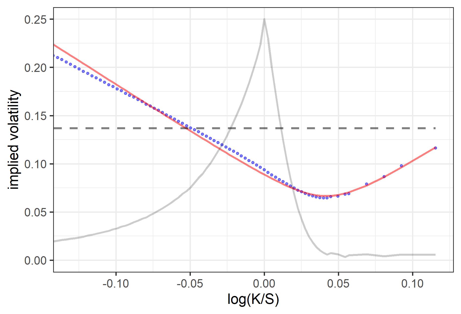
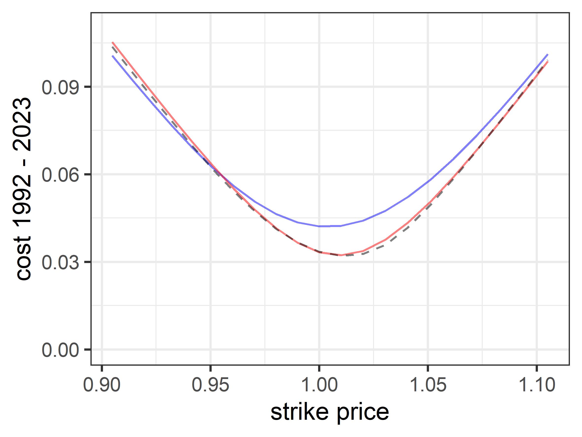
The field is in an exciting stage because quantum models are promising to offer new answers to key problems in economics and finance. For example, one of the oldest such problems is the pricing of options (those financial instruments which give the holder the right to buy or sell an asset at a future date for a set price). The classical theory of option pricing, which is based on the Black-Scholes model from 1973, has been described as the most accurate theory in economics, but the quantum model shows that for commonly-traded options and standard parameters it can be out by 40 percent. The fact that it still serves as the benchmark model is like a magic trick (see also here), where people don’t focus on the obvious flaws because they are distracted by the elegant and persuasive theory.

Advances in the field are also being driven by the development of quantum computing. Mainstream economics was shaped by the development of computers in the post-war era, and quantum computers are changing the way we think about the economy. For example, you can model the financial entanglement between a debtor and creditor as a quantum circuit, and similar circuits are used in quantum cognition to model how we make decisions, or in quantum computers to run artificial intelligence algorithms. Today a high school student can run quantum circuits to model the prisoner’s dilemma game which is new.

How has the way you understand the world changed over time, and what (or who) prompted the most significant shifts in your thinking?

There have been many changes and influences along the way, but to focus on one, my experience doing my D.Phil. on model error in weather forecasting changed the way that I thought about science and made me much more skeptical about things like incentives and the role of mathematical models. At the time there was a belief that weather models could be treated as essentially perfect so all error came from the inputs to the model – i.e. measurement of the current weather – amplified by chaos (the butterfly effect). This meant that forecasters just needed to run many forecasts from perturbed initial conditions, which of course required more computers and bigger budgets. Having worked already on some engineering projects, my view – and that of my supervisor Lenny Smith – was that the main problem wasn’t chaos or the butterfly effect, it was just that models were wrong, because you can’t build a perfect model of the weather. (It’s amusing how people are skeptical about things like quantum approaches, but unskeptical about models once they become established.)

Economics is an example of a field where the dominant ideas only make sense when you think of the incentives involved. During the Cold War, the promotion of results such as the Arrow-Debreu model of competitive equilibrium, which purported to prove the optimality of free markets, was as much about propaganda as science. The efficient market hypothesis – which states that prices adjust to new information immediately – is the economics equivalent of the perfect model hypothesis in weather forecasting because it assumes the equilibrium model is perfect. And mainstream economics, with its emphasis on efficiency, rationality, stability, and optimality, often sounds like the PR wing of the financial sector.

As with many other people (including a significant number of economics students), the 2007/8 crisis, when markets seemed less than stable or efficient, certainly changed the way I thought about economics. The Occupy Wall Street movement in 2011 was kicked off by Adbusters magazine, whose issue at the time featured an extract from my book Economyths, giving a call for economics students to overturn neoclassical orthodoxy and “do something new”. For me, that turned out to be quantum economics.

In recent years, James Der Derian initiated Project Q, Alexander Wendt published Quantum Mind and Social Science, and you are co-editor-in-chief of the new journal Quantum Economics and Finance. Is it fair to say that academia is starting to investigate the implications of quantum discoveries for the social sciences more seriously?

I had the pleasure of meeting Der Derian and Wendt at a quantum conference Wendt organised at Ohio State University in 2018. I really enjoyed the conference because everything seemed so wide open. It’s true that some in academia are starting to take quantum ideas a little more seriously but an interesting question is why it took so long (over a century!), and I would argue there has been a taboo on quantum which is only now being relaxed.

Part of this has to do with some physicists protecting what they see as their turf, but there seems to be a psychological or sociological component as well. One (not universally accepted) theory I put forward in a piece called “A softer economics” is that it relates to the role of gender.

The traditional, billiard-ball view of classical mechanics encodes stereotypically male values like solidity and certainty while quantum, which is based on wave functions and features uncertainty and entanglement, is more yin than yang. Some people get annoyed by the triteness of this idea but for me it seems reasonable, especially given the level of gender bias in both physics and economics. I suspect that if quantum had been discovered by women, instead of a group of young men, we would be calling it the most feminist theory ever. What happened though was that quantum was branded as quantum mechanics, and was considered okay for things like nuclear weapons, but if anyone tried to apply the ideas to human behaviour they were quickly slapped down.

In any case the fact that there has long been a taboo on the use of quantum outside physics, which has only recently been relaxed, is actually a real advantage for a new researcher because when such attitudes change, they tend to change quickly. Certainly, in economics, the number of people involved feels like it is in its exponential growth stage, which is why we decided to start a new journal.

Your new journal Quantum Economics and Finance sheds light on the use of quantum probability as a tool with which to illuminate our understanding of economics and finance. How is this achieved?

To give some background, related fields such as quantum cognition, quantum game theory, and quantum finance have been around for some decades, but there were no specialised journals, so people would end up publishing usually in physics journals where the topic was viewed as a sideshow. I saw the need to start a new journal while researching my book Quantum Economics, and teamed up with Emmanuel Haven who co-authored the book Quantum Social Science and set up the Centre for Quantum Social and Cognitive Science (CQSCS) at Memorial University.. Thanks to the team at Sage Publications we finally managed to get the QEF journal set up earlier this year (2023), with Ray Hawkins joining as managing editor soon after. Emmanuel started his academic career in finance and then went quantum, while Ray trained in quantum physics and then worked in finance, so we have all followed different paths. The editorial board has backgrounds encompassing economics, quantitative finance, mathematics, physics, quantum computing, complexity theory, game theory, psychology, and so on.

Quantum is from the Latin for “how much” and the idea of the journal is that quantum methods apply very well to the economy, where transactions are a way of answering the question “how much?”. The fuzzy notion of value is modelled as a wave function which when measured through transactions collapses down to a number, namely the price. This approach allows us to integrate the dynamical and probabilistic nature of decisions and transactions in a very natural way. In individual decisions, the wave function captures things like subjective factors which don’t appear in the classical analysis. In a model of the stock market, rotations of a quantum wave function represent the level of activity. (As a mental image, think of a skipping rope frozen in the shape of a bell curve. That’s classical probability, of the sort used in traditional theories like Black-Scholes. Now think of the same rope spinning around and distorting with speed, as if someone is actually skipping. That’s the quantum model.)

A basic question of course is whether the quantum approach is justified in an area like economics. The test of this is not whether we think it is permissible to adapt quantum ideas from physics, but a much harder one: it is whether, if the ideas had not existed, economists would have wanted to invent them. So, the aim is to produce models which meet that test, by making useful and accurate predictions.

Of course, what counts in economics is not just the mathematical models, but more broadly the underlying mental model of how things work, and here the quantum framework gives us a richer way of thinking about the economy as being made up of living, uncertain, entangled beings, rather than the classical picture of utility-optimizing “rational economic man”. And the area is very multidisciplinary. It’s interesting to see scientists from quantum computing firms teaming up with psychologists to model cognition, or a sociologist writing about the role of quantum social entanglement in the response to the climate crisis, or a physicist modelling retirement income.

Your proposed quantum approach offers a new insight outside the canon of International Relations to a neglected yet critical topic: the value of money. In what ways has money been overlooked in the study of international affairs?

As I argued in a paper for Security Dialogue, a main insight of the quantum approach is that money has an intrinsically dualistic nature, because it is a way to assign number to value, and these have incompatible properties (for example you can give someone a valuable object, but you can’t give them a number). As with quantum, there is unease around discussing money, and perhaps surprisingly this extends even, or especially, to the field of economics, where money is rarely discussed except as an inert metric, and topics like money creation were long treated as no-go areas, as researchers such as Richard Werner have pointed out.

When I submitted that paper an early reviewer seemed a little befuddled by what they described as a “detour” into the subject of money – even though money is obviously core to how countries interact (US power is related to the US dollar; and if you live in a country with an unstable currency, a dollar or a Euro is not an “inert metric” when you have to pay a debt in it). One thing is that academics working in the social sciences (with exceptions such as the late Susan Strange) may be uninterested in the topic of money, but also have a kind of grudging respect for economists so want to keep off their turf. But most economists have no clue about it either because it doesn’t fit into their classical worldview. In quantum economics, the complex, dualistic nature of money is taken as the starting point.

Could it be argued that information is analogous to money in the global system with the understanding that information is the fabric of the collective consciousness and international entanglement?

Yes, the emphasis on information is important, and it is what makes quantum an appropriate framework for the social sciences. As the quantum computer scientist Scott Aaronson (who is not involved in quantum economics) wrote, quantum probability is “about information and probabilities and observables, and how they relate to each other.” In physics, concepts such as superposition, interference and entanglement are applied to subatomic particles; in the social sciences, they are applied to ideas and information. For example, we can hold two ideas in our head at the same time, and they may interfere, or be entangled with other peoples’ ideas. Money is a particular form of information, which is used to collapse the fuzzy idea of value down to a hard number. There have been many theories of money, but most of these neglect its most basic property, which is its relationship to number.

Are there limitations of applying quantum ontology and methodology to the study of economics, finance, and IR?

Yes, our fascination with ontology is a problem! The interpretation of quantum physics is a topic of endless (if rather specialised) debate in physics. Quantum researchers in social science tend to follow one of two strands, which respond to this debate in different ways.

The first strand is to say that, according to some theories, the brain is based on quantum processes; so if that can be shown to be true, then it will follow that we are quantum and the social sciences need to be quantum too. However, while neurons may indeed turn out to exploit quantum effects, I find this argument to be rather reductionist, and don’t see what difference it would really make to a field such as economics: just because water is quantum doesn’t mean we expect plumbers to retrain in quantum mechanics, because what counts is the emergent properties. Or viewed the other way, the fact that a quantum model works well for something like the stock market doesn’t mean stocks are somehow ontologically at one with electrons.

The second strand, popular in quantum cognition, is the “quantum-like” approach which says we can borrow these models from physics because we are “like” a quantum system. This makes sense if you are trying to explain cognition using physical analogies, or drawing on advanced physics, but if you view quantum as a form of mathematics it doesn’t really work – we don’t say a systems dynamics model is planet-like just because calculus was first applied to planetary motion. And while a mathematical model is related to metaphor, it is different in that for example it can make specific predictions.

Either of these framings lead to confusion about what is “real”. For example, a typical comment (and a reasonable one from a physics perspective) is that a model isn’t “really” quantum because it does not describe “real quantum phenomena.” Yet for someone on a pay-day loan, the entanglement encoded by the information in the debt contract – which again can be written as a quantum circuit – seems pretty real. In general – and this probably comes more naturally to someone trained in the social rather than the physical sciences – information is real, even if it comes from a lawyer rather than the laws of the universe.

While quantum economics does draw on these and other interpretations, it therefore sees quantum probability primarily as a mathematical tool. To quote Aaronson again: “Quantum mechanics is what you would inevitably come up with if you started from probability theory, and then said, let’s try to generalize it so that the numbers we used to call ‘probabilities’ can be negative numbers. As such, the theory could have been invented by mathematicians in the 19th century without any input from experiment. It wasn’t, but it could have been.” It is interesting to think how things would have played out if quantum ideas had been adopted to study human behaviour before they were applied to physics – perhaps physicists would be worrying over whether it was intellectually defensible to model electrons as being like little people.

Again, the test of the quantum approach isn’t whether we have somehow inherited quantum properties such as superposition and entanglement from subatomic particles. Instead, the idea is more in the spirit of the first quantum pioneers, which is to take quantum social properties at face value, and use mathematics in a creative way to model observed phenomena. Viewed this way, attempts to relate everything to physics or create a unified ontology are something of a distraction. And we certainly have urgent problems where a quantum perspective would be useful. An example is the climate crisis, which could be viewed as the logical consequence of classical economics, the end result of individual utility-maximizing behaviour. One focus of the QEF journal is to investigate how quantum ideas can help loosen our doomed obsession with a particular type of economic growth.

In Economyths: 10 ways economics gets it wrong; you highlight the intellectual poverty of neo-classical economics. What are the ways in which economics gets it wrong?

The ten chapters in the original 2010 book were about ideas such as rationality, stability, individuality, and so on which characterise the classical picture of the economy (as opposed to the actual economy). The inspiration for this traditional view is often considered to be Newtonian science, but the ideas actually go back a lot further – in fact the chapter topics were based on a list of ten opposites from the Pythagoreans in ancient Greece. In a revised edition from 2017 I added an extra topic which combined aspects of the others, namely the (again, counterintuitive) fact that economics ignores or downplays the topic of money. This has left economists singularly unequipped to understand how much of the economy actually works. In Canada, for example, the economy is dominated by a housing bubble which economists try to analyse based on the mechanics of supply and demand, but is better understood from a quantum perspective as a money creation scheme – the financial version of a nuclear device – where the banks and some property owners are enriched, but the society as a whole is destabilised.

As Wendt noted in 2005 the same classical ideas have permeated the social sciences, and are backed up in part because of the (now somewhat tarnished) prestige of economics, which is associated with “hard” mathematics. So a first step for quantum economics is to build empirically-grounded alternatives to things like the “law of supply and demand”, the pricing of risk, and so on which out-perform the classical approach. Of course, not all models need to be quantum (and there is no such thing as a perfect model!), but together with other heterodox approaches like systems dynamics, complexity, ecological economics and so on the quantum approach can help reinvent economics. You don’t need to be a quantum expert to get involved.

How do you find inspiration to think innovatively and come up with unorthodox ideas, at the intersection of different academic disciplines?

One thing is that I trained in mathematics which allowed me to work across disciplines, including engineering, forecasting, systems biology, and economics (it probably helped that my jobs kept ending; for example, I returned to university after a particle accelerator project I was working on, the Superconducting Super Collider, was cancelled). However, another thing is the combination of science with writing for a general audience, which has been a great way to see topics from different angles. I credit this interest in part to familial influence – my father was an English professor – and also to my undergraduate university (Alberta) where mathematics could be taken as an arts subject, so I got to combine it with things like philosophy, art history, Shakespeare, film studies, and so on (even quantum physics). I also draw inspiration from my wife who as an architect works at the interface of art and engineering.

What would you say is the most important advice for a young scholar in IR?

I don’t really feel qualified to answer this one, but (since I’m here) I think the most important advice would be to NOT go into quantum. Sure, the methods can work. Yes, there are low-hanging fruit for early adopters. Okay, it is new and fun. And it is certainly true that the classical approach has failed, or at least run out of tarmac. But any rational person knows that it would be much better to keep in a safe, respected area rather than go down some weird and risky quantum path where the end point, if there is one, is highly uncertain. Of course, a few people will ignore this sensible advice, and we look forward to hearing about their work and maybe receiving their submissions at the journal.

See here for the original interview at E-IR.

CQF talk on a quantum view of Black-Scholes

It was a pleasure speaking yesterday at the Quant Insights conference marking the 50th anniversary of the Black-Scholes model. My talk presented nine predictions which came out of the quantum model – things that I had not been aware of, but that were suggested by the model and proved correct after empirical tests. And they all had implications for option pricing and the Black-Scholes model.

1. Before starting to work with the model, I didn’t know that price change and volatility for index data such as the S&P 500 or DJIA scale inversely with the square-root of time, even though the price change data is not normal, and volatility is not constant.

Density plots of log price changes, normalized by the square-root of time in years, for the S&P 500 over the years 1992-2021. The solid lines, from darkest to lightest shades of grey, are for periods of 1, 2, 4 and 8 weeks (measured in days). Dashed line is the quantum model.

2. I had heard of the square-root law of price impact, which says that the price change induced by a large order scales with the square-root of the order size, but didn’t know that the numerical coefficient was approximately one, as predicted by the quantum model.

Plot of price change versus order size Q over average daily volume V follows a square-root law with coefficient near unity.

3. I certainly didn’t know that the variance followed a simple equation that contradicted a published result.

Variance plotted against imbalance Q/(VT) where Q is order size, V is daily volume, and order time T ranges from 3.5 minutes (black) to 345 minutes (light grey). The single parameter sigma estimates the volatility.

The drawbacks of the neoclassical model of supply and demand have long been pointed out by critics such as Steve Keen. A basic one is that what counts is not supply and demand separately, but the ratio of demand to supply for available units. The quantum price impact model therefore gives an alternative model with only a single parameter, that has been rigorously tested for stock market data.

Plot of log price against imbalance, which is the ratio of demand to supply per available unit.

4. I had heard of the implied volatility smile in options trading, but didn’t know that actual volatility showed an even more pronounced smile, that followed a simple relationship with price change and time (and is related to price impact). I’m sure I am not the first person to notice this fact, but I haven’t seen it, or the connection with implied volatility, reported in the literature.

RMS annualized volatility for the S&P 500, plotted against normalized price change, for periods of 1, 2, 4 and 8 weeks (dark to light). Dashed line is the quantum prediction.

5. Implied volatility is not the same as actual volatility, because it is found by fitting a lognormal option pricing model to data that is not actually lognormal, and is affected by trader behaviour. So it was interesting to find that the quantum model produced an implied volatility surface very similar to what is found in the wild.

The quantum implied volatility surface is a somewhat flattened version of actual volatility.

6. The VIX index is an estimate of future volatility based on implied volatility, which is in turn used to price other options. The VIX is often described as being model independent, but its formula is based on two things: that volatility is independent of strike, and that the relevant growth rate is the risk-free rate. The former is an assumption of the Black-Scholes model, while the latter is its key finding. The VIX is therefore Black-Scholes in another guise. The quantum model predicted that the VIX substantially over-estimates both implied volatility and actual volatility, because its formula adds up the contributions of options in the wrong way. The results agree.

The VIX is produced using a formula which assigns weights to options (grey line) and produces a single volatility (dashed line) which is supposed to represent the implied volatilities (blue points). The quantum model (red) is a version of the smile curve.

7. Given that the Black-Scholes model assumes constant volatility, it makes sense that it should misprice options. However I for one was surprised to find that, according to the quantum model, it misprices at-the-money straddle options by a factor about equal to the square-root of two.

Comparison of straddle option pay-in for Black-Scholes model (blue) and quantum model (red), with expected pay-out (dashed). The Black-Scholes model misprices at-the-money straddles by about 40 percent.

8. Since the Black-Scholes model is the industry-standard pricing model, it makes sense that model error will lead to mispricing in option markets. This prediction was verified by Larry Richards who analyzed CBOE data for over 25,000 1-month SPX option prices from 2004 to 2017. So much for efficient markets. See our paper published in the March 2023 issue of Wilmott.

9. Finally, a logical consequence of this is that one can devise options-trading strategies to exploit this mispricing – for example, by selling at-the-money straddles (with appropriate protection to cover potential losses).

To summarise, the main difference between the classical random walk model traditionally used in quantitative finance, and the quantum model, is that the former assumes markets are at equilibrium and volatility is constant, while the latter treats markets as a dynamical system where price change and volatility are linked. The quantum model therefore does a better match of fitting and predicting market behaviour, without relying on additional made-up parameters of the sort so common in traditional quant finance.

In a panel discussion in which quants Emanuel Derman and Robert Litterman reminisced about the history of the Black-Scholes model, a viewer asked Derman whether “quantum economics and finance was too much of a stretch.” He agreed (again, predictably) that yes it was, without giving specific reasons (though he added that he would be willing to reconsider). And yet it’s strange that previous studies of implied volatility – including Derman’s own book The Volatility Smile – didn’t pick up on the obvious fact that the implied volatility smile is a weaker version of a smile seen in the actual asset price data (see my article The Black-Scholes Magic Trick in the July 2023 issue of Wilmott). Or that this would lead to a significant mispricing of commonly-traded options.

Models aren’t just tools to analyze systems, they also affect what we do and don’t see. And in finance, the quantum model isn’t too much of a stretch – it’s a perfect fit. For details of the quantum model, see here. And for more work along these lines, please follow our new journal Quantum Economics and Finance.

Update: A video of the talk is now available for members (free) at the CQF Institute website (see Part 3). See also the related paper “Quantum Uncertainty and the Black-Scholes Formula” available at SSRN.

The uncertainty principle, finance version

I’m a big fan of uncertainty. I’m more interested in what we don’t know than what we do know. In physics, that obviously leads naturally into quantum … where the idea of uncertainty is baked into the theory itself.
Shohini Ghose

In a Perimeter Institute podcast, quantum physicist Shohini Ghose discussed the role of uncertainty, applying it not just to physics, but to “questions around identity and society.” As she notes, “there is power to uncertainty, that the universe itself is telling us, stop with all of this precision measurements and stop with trying to know it all.” Despite the fact that quantum mechanics was developed over a century ago, “only recently have we really started exploring and digging deeply into the stranger properties of superposition, entanglement, all of which have quantum uncertainty underlying them.”

According to Ghose, there is a quantum revolution in the works which rivals the Industrial Revolution. The latter was shaped by a quest for precision and certainty in everything from production at scale to mass marketing. In contrast, “this whole new revolution with new quantum technologies” will reshape the way we think and behave. “Just like we move away in science from zero or one and go to zero and one, perhaps in society too, we will naturally start expanding our choices … and we will get to newer ways and newer approaches, which can influence so many aspects of our behavior.” (Listen to the full podcast here.)

While Ghose doesn’t discuss economics and finance, there is an interesting parallel with the world of quantitative finance.

This year marks the fiftieth anniversary of the Black-Scholes model, which is used to price financial options. The model has been described as “the most widely used formula, with embedded probabilities, in human history.” It is even more famous, though, for kickstarting the development of large-scale derivatives trading, by appearing to banish uncertainty from the pricing of options.

The Nobel-winning theory accomplished this by assuming that you can constantly buy and sell options and the underlying stock in such a way that the growth rate has to equal the rate of a risk-free instrument such as a government bond (so-called “dynamic hedging”). It was therefore unnecessary to make subjective and uncertain estimates of future growth. Key to the argument was that all the buying and selling will not incur excessive costs, and also that the volatility (standard deviation) of the price is a known constant.

In quantum economics, however, the bid/ask spread between buy and sell prices is not a technical detail, it is a fundamental level of uncertainty, and the main driver of volatility. The dynamic hedging proof therefore breaks down.

In a recent study that I carried out with hedge fund CTO Larry Richards, we showed that the key assumptions behind the Black-Scholes model do not hold up. Growth rates do matter, and they are uncertain. The volatility is not constant but depends on the degree of market imbalance, which affects the price change over an interval. The (empirically verified) result of all this is that, for commonly traded options, the Black-Scholes model is out by a factor about equal to the square-root of two.

The reason the Black-Scholes model has been so influential therefore is not because of its accuracy, but because it appeared to banish uncertainty from options trading, and transform it from what used to be considered a slightly disreputable form of gambling, into scientific risk management. In contrast, the new results came out of a quantum model of asset price behaviour which puts price uncertainty at its core.

In a sense, the two models therefore represent a different version of what we consider to be science. The Black-Scholes model appears to be rational and logical and certain. The quantum model takes uncertainty as its starting point. And the empirical evidence backs the latter.

So maybe, to borrow Ghose’s words, “the universe itself is telling us, stop with all of this precision measurements and stop with trying to know it all.” Finance is uncertain, and we can’t banish risk with an equation.

Why I’m a skeptic about quantum economics

Since I became involved in quantum economics, I have got used to hearing people announce that they are skeptical about the field. In the piece, I want to lay out the reasons why I too am skeptical.

Most people, when asked why they are skeptical, will point to physics envy, or compare the field with something flaky like quantum healing.

However, physics envy was identified as a problem in areas such as economics long before quantum ideas were being considered – it was just mechanistic physics rather than the quantum sort. And it is a little strange that the word “quantum” has flaky connotations (more on this below).

So these are not good reasons to be skeptical about quantum economics (for more along those lines, see here). My own reasons are different.

To start with, I am skeptical about mathematical models in general. My career in applied mathematics has had two main strands; building models, and pointing out the limitations of models. My D.Phil. was on the subject of model error in weather forecasting, and my first book was about why forecasts go wrong in a number of areas including weather, health, and economics. Other books explored the influence of aesthetics in physics, or the flawed assumptions behind the models used in economics and finance.

A common theme of these books is that complex systems such as the atmosphere or the economy resist prediction by mechanistic models, because they involve multiple interlocked (and often opposing) feedback loops, and because the number of unknown parameters explodes as more details are added. Highly sophisticated models can be built of anything from the climate system to the human heart, but the result is more of a movie-like simulation than a predictive model.

Quantum models are no exception to this rule. For example, a basic difference between classical and quantum probability is that the latter uses complex numbers (so parameters may have an imaginary component involving the square-root of negative one). The models are therefore much more flexible than classical models, just because every parameter has an imaginary component along with a real one. The fact that quantum models can do a good job of fitting complicated phenomena in fields such as psychology is therefore hardly surprising.

Another thing about mathematical models is that once they become accepted, they are surprisingly resistant to criticism. Economics in particular seems a safe space for models. An example is the Black-Scholes model for option pricing, which is still in use after 50 years despite its obvious flaws. From this perspective, a degree of skepticism is important, but people should reserve their strongest skepticism for established models, and be open to new ideas.

Finally, I am skeptical about arguments, of the sort sometimes heard in or around quantum social science, that the economy is quantum because the universe is quantum, or our minds are quantum. If the aim is to build a useful model of the economy, it isn’t much help to know that subatomic particles – and maybe mental processes – involve quantum interactions, any more than a weather forecaster would take these into account. And it would be very reductionist to conclude that, just because a simple quantum model can simulate a decision-making process, the process itself must be ultimately quantum.

However, being skeptical about such quantum applications is not an interesting or original position, it has been the default for about the last hundred years (although some founders of the field seemed open to the idea). The question is, why has it taken so long for these models to be properly explored? A skeptic might say that it has nothing to do with their accuracy, and is really about the fact that quantum seems to hold a special and carefully-protected place in the scientific psyche – which is one reason economic models have progressed little from the Victorian era.

Quantum probability is just the next simplest form of probability after the classical one, which is well-suited for handling the flow of information, and can accommodate properties such as superposition, interference and entanglement which characterize the economic world as much as they do the subatomic one. From the perspective of a mathematical modeler, quantum mathematics (including its use of those complex numbers) does seem to offer an appropriate structure for modeling a range of cognitive and economic phenomena. Most importantly, it can be used to provide useful insights and make accurate predictions about everything from our response to survey questions, to the price of financial options.

So, I consider myself a skeptic not just of quantum economics, but of all attempts to shoehorn the world into our neat mathematical equations. But I am also skeptical about the particular level of skepticism which is sometimes levelled against the application of quantum ideas outside of physics – especially from fields such as economics and finance where real, effective skepticism seems to be in such short supply.

Model blindness

Whether you can observe a thing or not depends on the theory which you use. It is the theory which decides what can be observed.

Albert Einstein, 1926

Mathematical models can be used to illuminate a system and make predictions about its behaviour, but they can also lead to a form of blindness.

A historic example is provided by supernovas, those massive stellar explosions which release a burst of radiation lasting months or even years. The first observations of such events by Western astronomers were in 1572 (recorded by the astronomer/alchemist Tycho Brahe) and then 1604 (recorded by his associate Johannes Kepler). However, Asian astronomers had known about them for centuries. The reason it took so long for the West to catch on was because astronomers there were blinded by Aristotelian science, which said that the planets rotated around the earth in spheres made of ether, and the heavens were immutable. Brahe also tracked a comet and showed that it would have smashed through those crystalline spheres, had they existed.

As I wrote in an article ten years ago, economics has its own versions of crystalline spheres which support its world view, and shape what is seen and not seen. One is Eugene Fama’s efficient market hypothesis, which states that markets immediately adjust to new information. The theory is reminiscent of Aristotelian physics, which assumed that in a vacuum changes take place instantaneously.

A related example is the random walk hypothesis, which assumes that asset prices are randomly perturbed at each time step, and which forms the basis of much of quantitative finance.

The nervous walk

The random walk model was first proposed by the French mathematician Louis Bachelier, whose 1900 dissertation on option pricing in the Paris Bourse described the behaviour of a stock’s price based only on its initial price, and the volatility (which Bachelier referred to as the “nervousness” of the stock). His thesis was initially ignored, but some 60 years later the economist Paul Samuelson found a copy “rotting in the library of the University of Paris,” and found it so interesting that he arranged for a translation. By 1973 the model had random walked its way to the heart of the developing field of quantitative finance, through the famous Black-Scholes model (also known as Black-Scholes-Merton or BSM).

The formula was based on the idea that one could construct a risk-free portfolio by dynamically buying and selling options and the underlying asset. Its “proof” relied on a number of simplifying assumptions, including efficient markets and the requirement that log prices follow the continuous version of a random walk with constant volatility. However its existence did seem to put option pricing onto a firm mathematical basis. Indeed, as Derman and Miller (2016) note, “the BSM model sounds so rational, and has such a strong grip on everyone’s imagination, that even people who don’t believe in its assumptions nevertheless use it to quote prices at which they are willing to trade.”

The continued strength of its hold is such that volatility in finance is usually assigned the dimension of inverse square-root of time (see for example Pohl et al., 2017) because this happens to hold for a random walk. But is this theoretical assumption justified?

Quantum conundrum

Unlike the classical model, the quantum model simulates price using a complex wave function which distorts when it is perturbed, leading to a change in volatility. It is therefore inconsistent with the classical assumption that volatility scales with the inverse square-root of time, which seems a bit of a conundrum until you remember that volatility is actually a relative (e.g. percentage) standard deviation so can be dimensionless.

I first became interested in this problem while investigating the question of how large transactions affect volatility. The quantum model predicts that the variance of price over the time T should be the sum of the normal volatility, which scales in the usual way with T, plus a term due to the order imbalance, which doesn’t:

Var = σ² T + σ² Q/(VT)

Here Q is the size of the excess order, V is volume per annum, σ is volatility, and T is the time period.

However when I checked the literature on market impact to see what else had been written on the topic, the best source I could find was a paper from a leading team of researchers which asserted that the variance in the square-root regime should follow the different formula

Var = σ² T + σ² a² Q/V

with “a as the only fitting parameter (a~0.1)” (though when I queried this value it was corrected to “around 3”). Since Q/V has units of time, this version was consistent with the orthodox assumption that σ² has units of inverse time.

A figure showed both “this prediction” and the actual variance as a function of Q/V for nine ranges of T, which seemed to give a good match – however the log-log scale of their graph made the results hard to interpret.

While I didn’t have direct access to the same data, the figure itself was already in the public domain, so after checking with the authors I digitalized the image to extract the points, and replotted with linear scaling (instead of log-log) as shown in Figure 1 below. With the linear scale it was obvious that the curves all have different slopes, with a variation from nearly 0 to around 5, and there is a distinct pattern where the slopes decrease with the duration T. The reason that the predictions lined up well with the data was because a different value of the tuning parameter was used for each line, so the model could effectively fit any slope at all. In other words, by any reasonable standard, the classical model clearly fails this empirical test (which of course has never been a deterrent to its use).

Figure 1. Variance as a function of Q/V for nine values of T from 3.5 to 345 minutes. The slopes show a clear inverse dependence on time T.

Market impact, fixed

Each curve in the original figure had a particular range of T, so using the mid-point of the range as the time duration, I plotted variance against Q/(VT) as per the quantum model (see Figure 2). Again, this version violates the assumption that volatility has dimensions of inverse square-root of time, however the slopes are now fairly constant with a mean of about 0.5. According to the quantum model this slope is not just a made-up fitting parameter but should provide an estimate for the volatility σ, so it is in the right range though somewhat higher. Given the inherent noisiness of the data, especially for smaller impacts, this confirms that the quantum model is capturing the underlying dynamics of market impact. I wrote the result up in a short note for Wilmott magazine.

Figure 2. Variance as a function of Q/(VT) for nine values of T from 3.5 to 345 minutes. The mean slope of the lines is about 0.5.

While the volatility of market impact might seem like a rather specialised topic, the common assumption that volatility can be treated as constant is in many ways the lynchpin of quantitative finance – take it away and the rest of the structure starts to look shaky. For example, as mentioned already it is a key assumption of the Black-Scholes model which controls the pricing of derivatives. And a related demonstration of model blindness – which has a great deal of practical importance – is the fact that the volatility smile seen in options trading has long been treated as a subjective quirk of traders rather than recognised as an intrinsic property of markets. More generally, the dynamics of market impact are also informative about the dynamics of supply and demand.

As empirical signals go, the discovery that volatility diverges from classical theory isn’t quite as spectacular as a supernova, but perhaps it will open some eyes to the fact that quantitative finance – and economics in general – is in need of some novel ideas.

References

Bucci F, Mastromatteo I, Benzaquen M, Bouchaud JP (2019 ) Impact is not just volatility. Quantitative Finance 19(11):1763-6.

Derman E, Miller MB (2016) The volatility smile. Hoboken, NJ: John Wiley & Sons.

Orrell D (2022) Market impact through a quantum lens. Wilmott 2022(122): 50-52.

Orrell D (2022a) A Quantum Oscillator Model of Stock Markets. Available at SSRN.

Orrell D (2022b) Keep on Smiling: Market Imbalance, Option Pricing, and the Volatility Smile. Available at SSRN.

Pohl M, Ristig A, Schachermayer W, Tangpi L (2017) The amazing power of dimensional analysis: Quantifying market impact. Market Microstructure and Liquidity 3(03n04):1850004.

Wilmott P, Orrell D (2017) The Money Formula: Dodgy Finance, Pseudo Science, and How Mathematicians Took Over the Markets. Chichester: Wiley.

QEF14 – Is the volatility smile real or imaginary?

The answer to this question, according to quantum finance, is both.

The volatility smile refers to the phenomenon in options trading where the implied volatility has a smile-like shape as a function of strike price (see Figure 1 below for an example). The volatility is lowest for at-the-money options where the strike price is the same (after discounting) as the current price, and is higher for out-of-the-money options.

The volatility smile is usually viewed as something of a conundrum, since it seems to violate the idea – which forms the basis of quantitative finance – that prices undergo a random walk with a volatility that can be described by a single number. The Black-Scholes model for option pricing, for example, assumes that prices follow a lognormal distribution with constant volatility.

This assumption is so widespread that in quantitative finance, volatility is usually expressed in terms of inverse square-root of time, because this happens to hold for a random walk where variance (i.e. volatility squared) increases linearly with time.

The quantum model differs from this classical random walk in a number of respects. In the classical model, a normal distribution is used to describe the possible range of prices at a particular time. This is an essentially static picture, which does not reflect the fact that price is the result of investors buying and selling, and assumes that markets are balanced. The quantum oscillator model replaces the normal distribution with a complex wave function, which rotates around the real axis. Since this is a dynamic model – the quantum version of a spring – it can be used to model this turnover process (it literally turns over in the imaginary plane), and capture what happens when markets are out of balance.

For example, a large order will perturb the price by an amount which depends on the square-root of the relative order size – which is just the well-known square-root law of market impact. However another effect is that the wave function also distorts in shape, leading to higher volatility.

In other words, market imbalance between buyers and sellers affects both price and volatility – so price and volatility are correlated, in a manner which happens to match the volatility smile seen in options trading.

Now, the volatility smile usually refers to the volatility that is implied by the price paid for options, so you could argue that it is based on traders’ subjective projections about the future, and is just a figment of their imagination.

But an easy way to test the hypothesis is to plot volatility versus price change for different time periods. For a lognormal distribution there is no correlation (and it is actually a bit tricky to produce an artificial data set which gives the right properties, but you can do it with the quantum model) but historical market data follows the predicted volatility equation.

Figure 1. Right panel shows volatility as measured by the VIX index versus monthly price change for the S&P 500 January 1992 to August 2022. Left panel is same for an artificial lognormal distribution. Red line shows average volatility, black line is the theoretical smile curve. The lognormal distribution shows no smile, while the market data smile is well approximated by the quantum formula.

Of course what we really care about here is the effect on option pricing. As mentioned, implied volatility usually refers to the volatility implied by the cost of options. But if the model is correct, then the cost should equal the expected payout. So another test is to ask, what volatility is implied – not by traders’ projections – but by after-the-fact market outcomes? In other words, what is the correct volatility to use in the Black-Scholes model so that the option cost calculated from the formula equals the expected payout, as determined from historical data?

The Black-Scholes model calculates option prices by assuming that the price distribution is lognormal. If the theory is correct, then the “market implied volatility” should be just the usual volatility, which does not depend on price change. The average option cost using this volatility should therefore equal the average payout (with of course an allowance for noise).

However the experiments show that while the Black-Scholes model does work for a lognormal data set – i.e. the model option cost equals the average payout – it produces systematic errors when historical data are used. It therefore fails a basic calibration test for a predictive model. Results can be improved by making volatility dependent on price change according to the smile equation.

Figure 2. Left panel shows Black-Scholes model cost (blue line) for 1-month straddle options, versus average payout for a lognormal distribution. Right panel shows the same for S&P 500 historical data. The red line shows the quantum model where volatility follows the smile curve. The Black-Scholes model is well calibrated for the artificial lognormal data, as expected, but the quantum model is a better fit for the market data.

So to summarize, the volatility smile is definitely real – even if the oscillations which produce it in the model take place in the imaginary plane.

For details, see the SSRN discussion papers:

A quantum oscillator model of stock markets

Keep on smiling: Market imbalance, option pricing, and the volatility smile

Previous: QEF13 – Quantum supply and demand

Playlist: Quantum Economics and Finance

Quantum economics FAQ

This post answers some questions that typically come up when discussing the quantum approach to economics and finance. For a list of broad objections (and responses) to the use of quantum probability outside of physics, see the post Ten reasons to (not) be quantum.

Why use quantum probability instead of classical probability?

The main difference between classical and quantum probability is that the former is based on yes or no, 0 or 1 logic, while the latter allows for superposition states (so yes and no, 0 and 1). This allows us to handle properties including interference and entanglement which characterize human interactions as much as they do the subatomic world. Another advantage of quantum probability is that it provides a useful framework for modelling probabilities that evolve dynamically (an example is the oscillator model of stock markets). Note also that quantum probability simulates a state using a complex-valued wave function, and much of its power comes from what has been called “the magic of complex numbers“.

How do quantum phenomena such as interference or entanglement occur in markets?

The field of quantum cognition models the decision-making process using the quantum formalism exactly because it can handle phenomena such as interference between incompatible beliefs, or entanglement between subjective context and objective calculations. Finance also has a more direct form of entanglement through things like debt contracts or the use of money.

Is this the same type of interference and entanglement as is seen in physical systems?

The point is that the same kind of model can be used for each. For example we can model a debt contract, including the potential decision to default, using an entanglement circuit on a quantum computer. The debtor’s decision is entangled with their subjective context; the creditor’s money is entangled with the debtor. Note that the entanglement involves information rather than macroscopic objects.

What are the practical applications of quantum economics?

Quantum economics offers an alternative to traditional economics that it is based on a different form of probability, and can be applied to a broad range of economic problems including decision making (quantum cognition), stock market analysis, option pricing, and the basics of supply and demand. More generally, it provides a mathematical framework for modelling properties such as subjectivity, interconnectedness, and power relationships which are downplayed or ignored in traditional economics.

Can the theory be used to make predictions?

The theory has been used to make a range of predictions (really postdictions, since the answer is known) including for cognitive effects of the sort studied in behavioural economics such as the order effect, the rate of strategic default on mortgages, the volume of options sold as a function of strike price, and the square-root law of market impact. One novel prediction was a relationship between price change and volatility that has important consequences for option pricing, since it violates a key assumption of the Black-Scholes formula.

Why is it appropriate to model social systems using concepts like force, mass and energy?

An advantage of quantum probability is that it provides a way to handle dynamical systems by quantizing forces. The entropic forces used in quantum economics are generated by propensity curves which specify the probability of an event such as a transaction. They are therefore just another way to describe a probability distribution, but they also serve as an intermediate step to create a quantum model. This in turn leads to natural definitions for concepts such as energy and mass, for example mass represents a resistance to change. Note that it is traditional in economics to talk about forces of supply and demand, but they are assumed to simply cancel out at equilibrium, so there is no need to describe something like mass.

Quantum systems are discrete, while observed systems are usually better described as continuous. For example a quantum harmonic oscillator has discrete energy levels, so how can we use that to model something like the price of a stock?

In the quantum model an oscillator represents a potential transaction. The energy level corresponds to the number of transactions over a time step, which is necessarily discrete (in a typical application the oscillator spends most of the time in the ground state, with transactions occurring every few steps). Indeed a defining feature of the economy is that it involves discrete transactions including money transfers.

What is the financial version of Planck’s constant?

In physics Planck’s constant is treated as an invariant quantity of nature, in quantum economics it is a parameter which decides the scaling for quantities such as mass.

Are quantum models more complicated than classical models?

The models used in traditional finance and economics are often very complicated because they need lots of bells and whistles in order to capture the complexities of the system. Quantum models do involve wave functions with an imaginary component, but the result can be simpler because they provide a more natural fit in the first place. For example in the oscillator model, the ground state is a wave function which rotates around the real axis and acts as a counter for transactions, which is only possible because it has an imaginary component. The only extra parameter is the oscillator frequency, which is needed in any case to describe the frequency of transactions.

Do you need a degree in quantum mechanics in order to work in this field?

No, most of the mathematics is basic linear algebra or calculus. In fact, while physicists tend to be the go-to experts for tricky technical problems, a training in physics sometimes seems to be a blocker – for example physicists often struggle with the idea of social or financial entanglement because they want to relate it to the behaviour of subatomic particles, instead of just looking at the math.

What is the difference between quantum economics as described here, and other quantum approaches?

Quantum economics starts with the idea that money has complex dualistic properties which are best handled using a quantum approach. It draws on ideas from quantum cognition and quantum finance, which developed independently. One approach to quantum finance is to see it just as a mathematical tool for solving hard problems from traditional quantitative finance (such as derivative valuation), without any attempt to incorporate effects such as interference or entanglement (for a critique see here). Another is the “quantum-like” approach which transposes models from physics, without necessarily trying to justify them from basic principles. Finally there is the two-state approach which focuses on price, and models stock markets in terms of a price operator with two states representing the bid and the offer. In this view, there is no concept of force or mass (instead mass is subsumed in the definition of the financial Planck’s constant). Quantum economics differs from the first in that it is concerned with quantum phenomena such as interference and entanglement; from the second (slightly) in that it derives models as far as possible from first principles rather than importing then from quantum physics; and from the third in that concepts such as force and mass are viewed as useful components of the model (however two-state models can be derived from it). Quantum economics is therefore broadly compatible with these other approaches, but treats mental and financial phenomena as quantum in their own right.

Does quantum economics assume a direct link with quantum mechanics, for example through quantum processes in the brain?

No, and even if consciousness turns out to rely on quantum processes we couldn’t infer from it that the economy should be modelled using wave equations. Similarly, the fact that quantum models are useful for modelling human cognition does not imply that the brain is quantum. In quantum economics, we take social properties such as interference and entanglement at face value rather than arguing that they are inherited from subatomic particles. The test of quantum probability in economics is not whether its use can be justified by physics; it is whether, if it had no known application in physics, we would still want to use it to model social systems.

Where can I receive training in quantum economics?

Quantum economics and finance has been chosen as a thesis topic by a number of students in higher education. Memorial University in Newfoundland has set up a Centre for Quantum Social and Cognitive Science whose remit includes quantum economics. People who wish to get into the area can check out a number of online resources including the papers here or for a general introduction this video series.

QEF13 – Quantum supply and demand

The neoclassical X-shaped supply and demand diagram is featured in every introductory textbook, is the basis for mathematical models of the economy, and has shaped our view of the economy for over a century, but as critics have pointed out many times it has a few basic problems (see Economyths for a summary).

It assumes static equilibrium so there is no dynamics. Supply and demand are assumed to be independent, when we know they are often coupled. And finally, there is no empirical validation for the diagram. For example demand curves involve hypothetical transactions which we can never observe. We also know that prices are not drawn to a stable equilibrium, but are subject to complex dynamics.

The quantum version starts by observing that supply and demand are two sides of the same coin, so what counts is the degree of imbalance – if both increase at the same time it has no effect on price (at least to first order). Modelling potential transactions with a quantum oscillator then leads to a version of the square-root formula derived for price impact in QEF12.

To start with a simple illustration, consider a scenario where there is one seller and one buyer for some perishable item such as a loaf of bread. The seller wants to sell one unit per day, and the buyer wants to buy one unit per day, so the system is balanced. We can model this using an oscillator in the ground state, where the wave function rotates around the real axis with a frequency of once per day, and the squared amplitude representing the joint propensity function is a normal curve.

Suppose now that another buyer enters the picture. The expected transaction rate will therefore double, and the supplier may not be able to keep up. In order to restore the original frequency, the required price increase from the formula is x=√2 σ where σ measures the degree of price flexibility. Making this change requires energy ∆E=ℏω∕2. As mentioned in QEF09 this is the base quantum of energy which allows for the possibility of a transaction between two people. The energy added by increasing the frequency is therefore balanced by the energy spent in increasing the price.

Left panel shows the probability distribution for the oscillator in the ground state. Adding an additional buyer shifts the oscillator to the right (as indicated by arrow). Right panel depicts the complex wave function rotating around the real axis.

In the general case, define the imbalance to be ι = (Nb – Na )/min⁡(Na,Nb ) where Na is the number of sellers and Nb is the number of buyers. As with the price impact result from QEF12, we then get a change in log price of x=±Yσ√|ι| where Y=√2 and the sign depends on the sign of ι. This formula is shown in the right panel of the figure below.

Left panel shows the neoclassical supply and demand diagram. Source: Instant Economics. Right panel shows the quantum version with the uncertainty parameter set to σ=0.02. Change in log price has a square-root dependency on the demand/supply imbalance ι. The shaded area, representing price uncertainty, shows one standard deviation.

Another feature of the quantum oscillator model is that volatility is a function of the energy level, so if the energy state is En then the volatility will be σn=σ√(2n+1)=σ√(|ι|+1). It follows that observed volatility is not a constant, as usually assumed in finance, but varies depending on energy level. The uncertainty therefore increases with the degree of market imbalance, which is consistent with the large fluctuations seen during times of market stress.

If we assume the model is perturbed at each step by an amount ∆x=σ as in QEF12, then the energy of the system follows a Poisson distribution with average given by λ=1/4. This modifies the multiplicative constant for the price impact formula slightly to Y=√(4/3) which is in the correct range.

To summarise:

• The quantum model treats supply and demand, not as fixed or independent, but as two coupled aspects of a single dynamic process

• Transactions are inherently probabilistic – the uncertainty parameter σ is not an external noise term or addition, but is integral to the formula

• The model responds dynamically to perturbations, and produces non-Gaussian statistics due to changing volatility

• The model predicts (or postdicts) the square-root law of price impact, including a value for the multiplicative constant

For details, see the SSRN discussion paper Quantum impact and the supply-demand curve.

Previous: QEF12 – A quantum oscillator model of stock markets

Playlist: Quantum Economics and Finance